Tip of the Week - Spot Risky Sales with Conditional Formatting
In Zoho Analytics, small tweaks can lead to big insights. One such feature is Conditional formatting based on other columns, your key to instantly spotting where sales success is overshadowed by product returns.
Our tip this week shows you how to apply conditional formatting across columns to uncover products and categories that look like top performers in sales but reveal a different story once returns are factored in.

The Big Picture
High sales don’t always mean healthy business. A category may dominate revenue, but if product return rates are unusually high, your profits and customer trust take a hit. Looking only at sales hides this risk.
Conditional formatting based on return rates bridges that gap. It helps you go beyond surface numbers and focus on product quality and customer experience.
In this demo, we’ll start with a pivot table arranged as follows:
Columns: Month
Rows: Product Category
Data: Sales (USD), Return Rate (%)
Get ready to see how sales dominance changes month to month and how return rates reveal a deeper layer of truth.
We’ll highlight three eye-catching zones using conditional formatting:
- Healthy Zone - Low returns
- Warning Zone - Rising returns
- Critical Risk - Unacceptable return rates
By the end of this demo, sales won’t just be tall bars on your pivot; they’ll instantly tell you which categories are fueling sustainable growth, and which ones are silently eroding your margins.
Check out the video here:
Steps to Apply
- Open your Pivot Table.
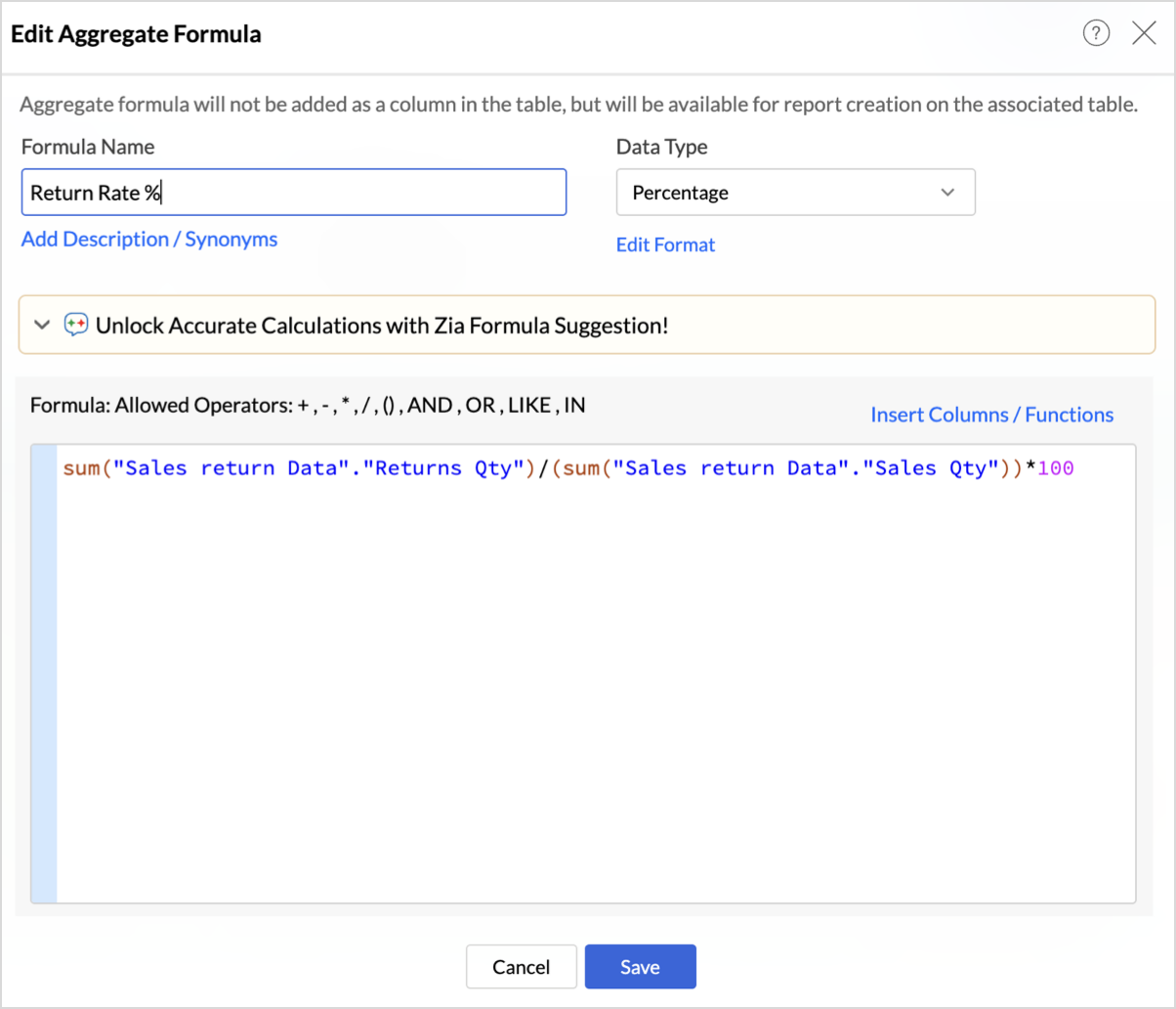
- Creating Return Rate Formula:
- Click Add Aggregate Formula.
- Enter Formula name as Return Rate.
- Define the metric as below:
- Click Save.
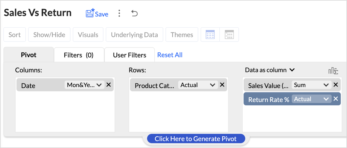
- Set up your pivot table as shown below.
- Columns: Month
- Rows: Product Category
- Data: Sales (USD), Return Rate (%)
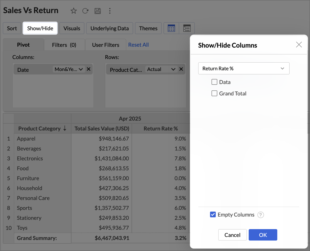
- Hide the Return Rate % column from the pivot as shown below.
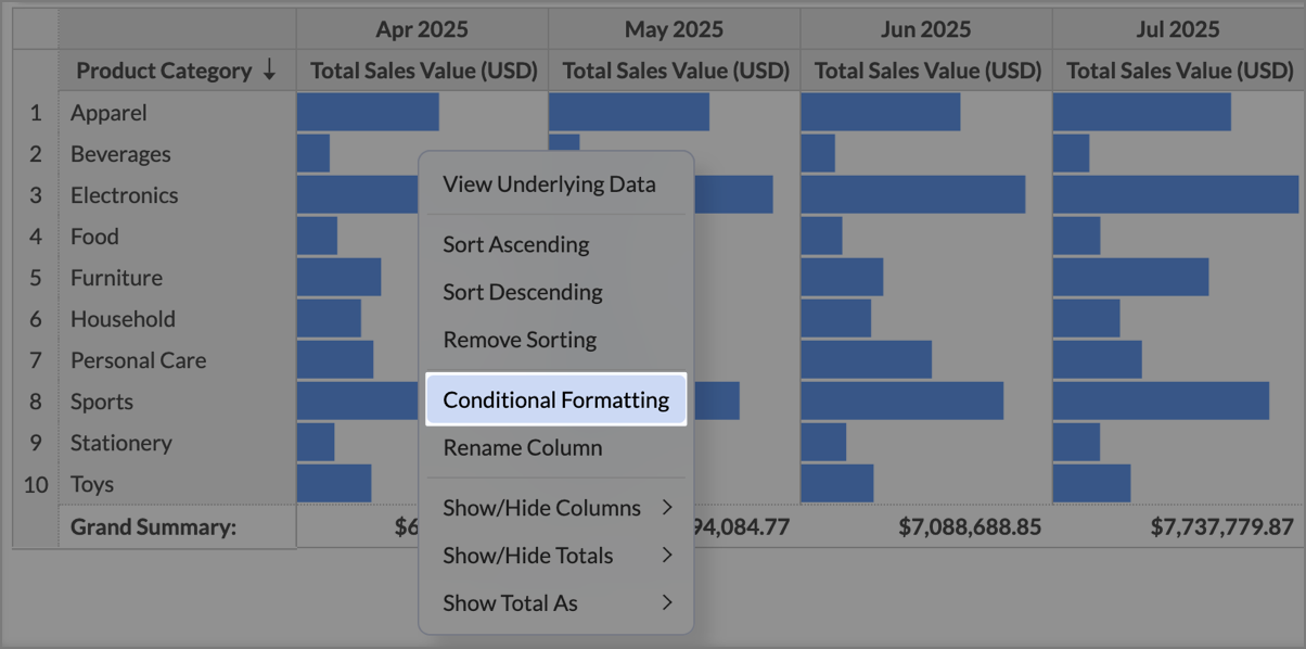
- Click Visuals and select Only Data Bars.
- Right-click on any Sales cell and select Conditional Formatting.
- In the Conditional Formatting dialog, under Based On, choose Return Rate (%).
- Define three conditions based on the following zones:
- Critical Risk - Set the condition as Greater than or Equal to 10 and choose Red fill in Additional Formatting options.
- Warning Zone - Set the condition as Between 5 to 10 and choose Amber fill.
- Healthy Zone - Set the condition as Less Than or Equal To 5 to 10 and choose Amber fill.
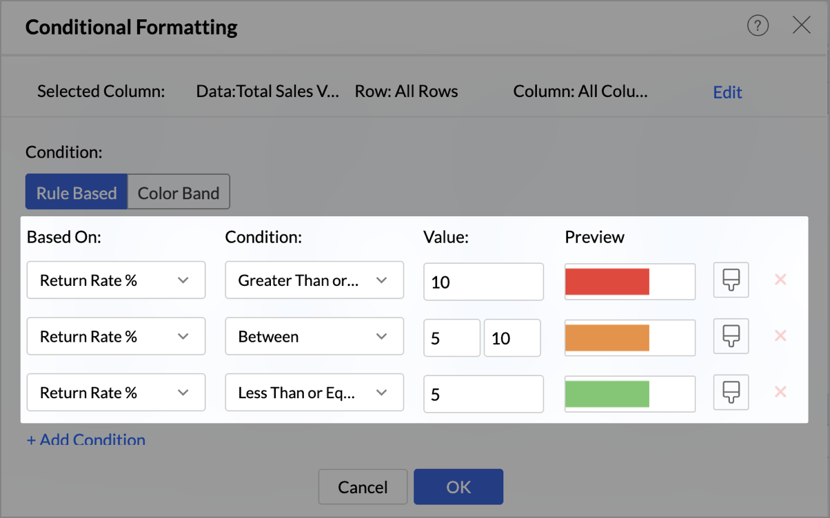
- Click OK to save the conditions.
sum("Sales return Data"."Returns Qty")/(sum("Sales return Data"."Sales Qty"))*100
This formula calculates the percentage of sold items that were returned, giving you the Return Rate % for each product category and month in your pivot.
What you should see
- Green Sales Bars where return rates are low → sustainable business.
- Amber Bars where returns are rising → early warning.
- Red Bars where sales are hit by high returns → high-priority fix.

With one glance, your pivot now tells a double story: who’s leading in sales and who’s at risk due to high returns.
Best Practices
- Highlight what matters most: Focus on key risk signals like high return rates or unexpected spikes. This keeps the pivot sharp and attention where it belongs.
- Use KPI-driven thresholds: Base your rules on meaningful KPIs (like Profit Margin % or Return Rate %), not arbitrary numbers. This ensures the colors always map to business impact.
- Keep colors intuitive: Stick to natural associations: Green = Healthy, Red = Risk, Orange = Caution. This makes insights instantly recognizable for everyone.
- Pair visuals for impact: Don’t stop at colors. Combine conditional formatting with Data Bars to highlight magnitude, or Sparklines to reveal trends over time. Layering visuals makes patterns clearer without adding extra clutter.
- Test across different data ranges: For broader cues, try Color Bands to show intensity (like a heatmap of return rates) or Icon Bands to flag quick signals
- Avoid overlapping rules: Overlaps can confuse users. Keep each condition distinct to avoid conflicting colors on the same cell.
- Explore Color Bands and Icon Bands: If you want a broader visual cue beyond rule-based formatting, try Color Band (gradient shades that show intensity, like heatmaps) or Icon Band (symbols that signal performance trends). These are especially effective where quick scanning matters more than raw numbers.
- Think ahead for storytelling: Design your formatting with the end reader in mind. The goal isn’t to decorate numbers; it’s to tell a story at first glance.
When done right, conditional formatting turns pivots into a decision board. Your wins glow green, your risks flash red, and your opportunities pop out without a single extra click.
Keep Exploring
- Help Documentation
- Help Videos
Topic Participants
Pradeepkumar R
Sticky Posts
Tip of the Week - Spot Risky Sales with Conditional Formatting
In Zoho Analytics, small tweaks can lead to big insights. One such feature is Conditional formatting based on other columns, your key to instantly spotting where sales success is overshadowed by product returns. Our tip this week shows you how to apply
Recent Topics
A new UI for distraction-free engagement in online meetings and webinars that scale up for 3000 attendees
Hello all, We're excited to share our new, refined UI for online meetings. Here's how the new UI will improve your experience during online meetings: We've re-designed Zoho Meeting's online meeting UI to enable users to fully engage in conversationsLatest updates in Zoho Meeting | Create departments, Share PDF files
Hello all, You can now create departments to group team members within your organization. This will make it easier for you to organize department-level meetings and invite members. In webinars, use the Share material feature to share PDF files directlySupport “Never End” Option for Recurring Meetings in Zoho Meeting
Hello Zoho Meeting Team, Hope you are doing well. We would like to request support for creating recurring meetings with no end date in Zoho Meeting. Currently, when scheduling a recurring meeting, Zoho Meeting requires us to select a specific end date.Direct “Add to Google Calendar” Option in Zoho Meeting
Hello Zoho Meeting Team, Hope you are doing well. We would like to request an enhancement related to the “Add to Calendar” functionality in Zoho Meeting. Currently, when we open Zoho Meeting and view our meetings under My Calendar, there is an Add toI Can't Clone Webinar that I Co-Organize
How do i get our account admin to give me permission to clone our webinars? I am a co-organizerUnify All Zoho Video Meeting Experiences into One Standardized Platform
Hi Zoho Team, We would like to share an important user experience concern regarding the current state of video meeting functionality across the Zoho ecosystem. The Problem Within Zoho, there are multiple ways to initiate or schedule a video meeting: ZohoLatest updates in Zoho Meeting | Calendar view, Zia integration with OpenAI, edit the recurring pattern in a recurring meeting, device error notifications revamp, and more.
Hello everyone, We’re glad to share a few updates and enhancements in Zoho Meeting, including the Calendar view, being able to edit the recurring pattern in a recurring meeting, revamped device error notifications, and other enhancements that you’ll findNew enhancements in the latest version of the Zoho Meeting Android mobile app.
Hello all, In the latest version of Zoho meeting Android mobile app (v2.2.6), we have brought in support for the below enhancements. Close account: Now users will be able to close their Zoho account directly from the app. Unmute toast message: If a userShare material, Lock Meeting and revamped feedback UI in the latest version of the Meeting iOS app.
Hello all, In the latest version of the Zoho Meeting iOS mobile app (v1.6), we have brought in the below enhancements. Share material in meeting: We have introduced share material during meeting that allows participants to view supported materials suchLatest updates in Zoho Meeting | New chat feature between an organizer and co-organizer in webinars, recording consent for webinar co-organizers and attendees in the Android app, and more.
Hello everyone, We’re excited to share a few updates for Zoho Meeting. Here's what we've been working on lately: A new chat feature between an organizer and co-organizer in webinars, recording consent for webinar co-organizers and attendees in the AndroidLatest updates in Zoho Meeting | A new Files tab to manage all your PDFs, PPTs, Video files and recordings, live transcription , ability to lock settings and adaptive echo cancellation.
Hello everyone, We’re excited to share a few updates for Zoho Meeting. Here's what we've been working on lately: A new Files tab to manage all your PDFs, PPTs, Video files and recordings, live transcription during sessions, ability to lock settings andLatest updates in Zoho Meeting | Meeting Rooms , Pin video feeds and customize from and reply-to email addresses
Hello everyone, We’re excited to share a few updates for Zoho Meeting. Here's what we've been working on lately: Introducing Zoho Meeting Rooms, an immersive solution for teams to connect over virtual meetings in video conference rooms. You can also pinLatest updates in Zoho Meeting | New top bar video layout, a revamp of our in-session settings and now import webinar registrations with a CSV file
Hello everyone, We’re excited to share a few updates for Zoho Meeting. Here's are some of them : We have moved audio, video, virtual background and preferences under a single settings pop-up for better user navigation. You can now upload a CSV file containingLatest updates in Zoho Meeting | New End of session notification to remind everyone about the session end time
Hello everyone, We’re excited to share a new feature for Zoho Meeting ; End of session notification. With this new setting, you can choose to remind all participants or only the host about the scheduled end time of a meeting. You can also choose whenImportant update: Changes in email sender policies
Hello, This is to announce important changes to email sender policies from Google that may impact your use of Zoho Meeting. Restriction on public domains Effective February 1, 2024, Google is implementing policies that will affect the configuration ofCamera access
My picture doesn't appear in a group discussion. (The audio is fine.) The guide says "Click the lock icon on address bar," but I can't find it. Advise, pleaseChat for webinar session, schedule meeting session for 24 hours - Zoho Meeting iOS app update
Hello, everyone! In the most recent iOS version of the Zoho Meeting app, we have introduced the chat functionality for the webinar session. To access this feature, the Organizer should have the 'Public chat' option enabled on the Zoho Meeting desktopInvoice Copy 2005116990189
Please provide the invoice for the trancaction 2005116990189Darshan Hiranandani About
Hi, I’m Darshan Hiranandani, a dedicated software developer with a strong passion for creating efficient and user-friendly applications. With a degree in Computer Science and several years of experience in the tech industry, I specialize in full-stackLatest update in Zoho Meeting | On-demand webinars
Hello everyone, We’re excited to introduce our new on-demand webinar feature, you can now provide pre-recorded sessions that your audience can access immediately, no need to wait for scheduled sessions. Benefits of On-demand webinars : Scheduling flexibilityZoho Meeting iOS app update - Join breakout rooms, access polls, paste links and join sessions, in session host controls
Hello, everyone! In the latest iOS version(v1.7) of the Zoho Meeting app, we have brought in support for the following features: Polls in meeting session Join Breakout rooms Paste link in join meeting screen Foreign time zone in the meeting details screen.Zoho Meeting app update.
Hello, everyone! In the latest Android (v2.3.7) and iOS (v1.7.1) versions of the Zoho Meeting app, we have brought in support for the following features: Report Abuse option. WorkDrive integration. Report Abuse option You can now report to us any deceptiveZoho Meeting Android app update - v2.4.0
Hello everyone! We are excited to announce that we have brought in support for the following features in the latest version of the Zoho Meeting Android app(v2.4.0): 1. Start Personal Meeting Rooms 2. Revamp of the schedule meeting screen and meeting detailsIntroducing Zoho Desk integration and a few minor enhancements
Zoho Desk Integration We've now introduced an integration between Zoho Meeting and Zoho Desk to efficiently manage meeting-related customer inquiries. With this integration, you can track, respond to, and resolve meeting-related tickets directly fromZoho Meeting iOS app update: Hearing aid, bluetooth car audio and AirPlay audio support.
Hello everyone! We are excited to announce the below new features in the latest iOS update(v1.7.4) of the Zoho Meeting app: 1. Hearing aid support: Hearing aid support has been integrated into the application. 2. Bluetooth car Audio, AirPlay audio support:Zoho Meeting Android app update: Breakout rooms, noise cancellation
Hello everyone! In the latest version(v2.6.1) of the Zoho Meeting app update, we have brought in support for the following features: 1. Join Breakout rooms. 2. Noise cancellation Join Breakout rooms. Breakout Rooms are virtual rooms created within a meetingiOS 12 update: Introducing autofill passwords and Siri Shortcuts in Zoho Vault
With this iOS 12 release, Zoho Vault users can now autofill usernames and passwords on Safari and other third-party apps. Users can enjoy a seamless login experience to their everyday apps without compromising security and also access passwords stored in Zoho vault with Siri Shortcuts by adding personalized phrases. How to enable autofill password on your iOS device? First, you need to update your device to iOS 12. Apple recommends you to take a backup before you update your device to the latestZoho Vault: A look at what's new for iOS, iPadOS, and macOS
Hi everyone, At Zoho Vault, we constantly aim to improve your security experience. Based on both internal and external feedback, we have recently rolled out updates across our iOS, iPadOS, and support for macOS platforms. Introducing the desktop app forBiometric Access Support on Zoho Vault Desktop App
Is there any plans to add biometric authentication (fingerprint, face recognition) for Vault desktop apps (Windows/macOS) to enhance security and ease of access. I would love to hear other members view on thisFree webinar: Learn the benefits of migrating to Zoho Vault's new interface
With remote work becoming more and more common across the globe, productivity and time management are now pivotal concerns for every organization. With the number of business applications employed by companies constantly increasing, a password manager like Zoho Vault saves a lot of productive hours for your team. Vault's new interface has been carefully designed to address these pressing needs, helping users increase their productivity while improving their overall online experience. This July,Free Webinar: An exclusive live Q&A session with the Zoho Vault team
As 2020 draws to an end, we're closing out a year that has seen drastic changes all around the world. Many businesses have adopted cloud solutions and a remote work culture for the first time, and this has given rise to newer cyber risks and threats thatWhy passwordless authentication should be your top security project for 2021
Hello users! We know that nobody likes to remember passwords, yet they form an indispensable part of our lives. Many of us working with any kind of technology today manage numerous passwords for personal and business accounts. With the widespread adoptionFree Webinar: See why Zoho Vault is the best alternative to LastPass
When LastPass was acquired by LogMeIn in Oct 2015, we expressed our genuine concern about how this would change the LastPass business model and how customer trust would transfer from one company to another. As we suspected, LastPass doubled their pricingManaging cyber threats when working remotely | A Customer Survey Report
The nearly universal adoption of remote work has changed the way businesses function. Globally, enterprises continue to work to find new ways to make life easier for employees working remotely. However, a commonly cited concern has been the lack of cybersecurityWorld Password Day: 5 interesting facts about passwords
It's World Password Day: that time of the year when we talk about password hygiene and the importance of safe password management. World Password Day is observed on the first Thursday of every May, and this year, we'd like to talk about some of the mostFree Webinar: Go passwordless in 2022 with Zoho Vault
Passwords have long been the preferred authentication method, largely due to their universal appeal. While they're easy for people to use and implement, they're also convenient for hackers to exploit. Reports from 2021 state that weak and stolen passwordsMyki has announced EOL for its services | Learn why Zoho Vault password manager is the best alternative
Hello Myki users, Myki has announced end-of-life for its Teams, MSP, and GUARD services, after being acquired by JumpCloud. In their recent announcement, Myki stated that they will be removing their apps and extensions from the respective stores, turningJoin our exclusive meetup with Zoho's Real Estate community
Hey there, The Zoho Vault team is conducting a meetup for all real-estate users from Zoho. During this session, we will be discussing the need for secure password management and how Vault can help you and your clients safely protect passwords and otherFree webinar: A quick walkthrough of Zoho Vault and major updates in 2023
Managing passwords is crucial for all businesses. You can securely store, share, and manage passwords effectively from anywhere with Zoho Vault. We have introduced several new features in 2023 to offer the best online experience for our users. Join ourFree webinar: Why a password manager is a “must-have” for everyone in 2024
In the past decade, we've witnessed numerous cybersecurity breaches globally, with a significant portion resulting from the "it won't happen to me" mindset. Shockingly, in 2023, 86% of breaches involved weak and stolen passwords. Password hygiene is crucialNext Page